Working with Maps and GIS data
Notable packages
The tidycensus packages
- Website: https://walkerke.github.io/tidycensus/
- Install with
install.packages("tidycensus") - Vignettes: https://walkerke.github.io/tidycensus/articles/basic-usage.html
- Reference: https://walkerke.github.io/tidycensus/reference/index.html
The simple feature packages
- Website: https://github.com/r-spatial/sf
- Install with
install.packages("sf")- On Mac, you may need to install
udunitsfirst, for example, with homebrew - On Linux, install
libudunits2-devwith your software management system first
- On Mac, you may need to install
- Vignettes: https://r-spatial.github.io/sf/articles/sf1.html
- Reference: https://r-spatial.github.io/sf/reference/index.html
Code examples
Data files used in the examples
- Portland Metro 1994 TAZ shape file: Download & unzip to
datasubdirectory of your RStudio project folder - Portland Metro 1994 Survey geocode.raw.zip
Map ACS 2012-16 Median Household Income by Census Tract
## Install the tidycensus package if you haven't yet
#install.packages("tidycensus")

library(tidycensus)
library(ggplot2)
library(dplyr)

## setup cenus api key
## signup your census api key at http://api.census.gov/data/key_signup.html
census_api_key("5d1693be6ce12231248f292759f241c1ead3ed53") # note: needed to re-build website
## To install your API key for use in future sessions, run this function with `install = TRUE`.portland_tract_medhhinc <- get_acs(geography = "tract",
year = 2016, # 2012-2016
variables = "B19013_001", # Median Household Income in the Past 12 Months
state = "OR",
county = c("Multnomah County", "Washington County", "Clackamas County"),
geometry = TRUE) # load geometry/gis info## Getting data from the 2012-2016 5-year ACS## Downloading feature geometry from the Census website. To cache shapefiles for use in future sessions, set `options(tigris_use_cache = TRUE)`.##
|
| | 0%
|
|= | 2%
|
|== | 3%
|
|=== | 4%
|
|=== | 5%
|
|==== | 7%
|
|===== | 8%
|
|====== | 10%
|
|======= | 11%
|
|======== | 12%
|
|========= | 13%
|
|========== | 15%
|
|=========== | 16%
|
|============ | 18%
|
|============ | 19%
|
|============= | 20%
|
|============== | 22%
|
|=============== | 23%
|
|================ | 24%
|
|================= | 26%
|
|================== | 27%
|
|=================== | 29%
|
|=================== | 30%
|
|==================== | 31%
|
|===================== | 33%
|
|====================== | 34%
|
|======================= | 35%
|
|======================== | 37%
|
|========================= | 38%
|
|========================== | 41%
|
|=========================== | 42%
|
|============================ | 43%
|
|============================= | 45%
|
|============================== | 46%
|
|=============================== | 48%
|
|================================ | 49%
|
|================================= | 50%
|
|================================== | 52%
|
|=================================== | 53%
|
|=================================== | 54%
|
|==================================== | 56%
|
|===================================== | 57%
|
|====================================== | 59%
|
|======================================= | 60%
|
|======================================== | 61%
|
|========================================= | 63%
|
|========================================== | 64%
|
|========================================== | 65%
|
|=========================================== | 67%
|
|============================================ | 68%
|
|============================================== | 71%
|
|=============================================== | 72%
|
|================================================ | 73%
|
|================================================= | 75%
|
|================================================== | 76%
|
|=================================================== | 78%
|
|=================================================== | 79%
|
|==================================================== | 81%
|
|===================================================== | 82%
|
|====================================================== | 83%
|
|======================================================= | 84%
|
|======================================================== | 86%
|
|========================================================= | 87%
|
|========================================================== | 89%
|
|========================================================== | 90%
|
|=========================================================== | 91%
|
|============================================================ | 93%
|
|============================================================= | 94%
|
|============================================================== | 95%
|
|=============================================================== | 97%
|
|================================================================ | 98%
|
|=================================================================| 100%(myplot <- ggplot(portland_tract_medhhinc) +
geom_sf(aes(fill = estimate)) +
coord_sf(datum = NA) + theme_minimal())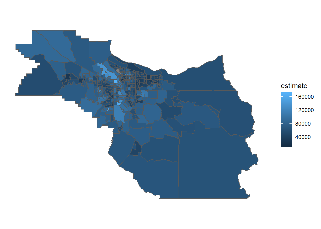
#ggsave("output/mymap.pdf", myplot)Interactive Maps of ACS 2012-16 Median Household Income by Census Tract
## Install the mapview package if you haven't yet
#install.packages("mapview")
library(sf)
## Linking to GEOS 3.6.1, GDAL 2.2.3, PROJ 4.9.3library(mapview)
library(dplyr)
mapview(portland_tract_medhhinc %>% select(estimate),
col.regions = sf.colors(10), alpha = 0.1)Example of spatial analysis: spatial join
library(sf)
library(readr)
# read 1994 Metro TAZ shape file
taz_sf <- st_read("data/taz1260.shp", crs=2913)
## Reading layer `taz1260' from data source `C:\Users\jbroach\Projects\datasci\datascience2019\data\taz1260.shp' using driver `ESRI Shapefile'## Warning: st_crs<- : replacing crs does not reproject data; use st_transform
## for that## Simple feature collection with 1247 features and 1 field
## geometry type: POLYGON
## dimension: XY
## bbox: xmin: 7435706 ymin: 447796.5 xmax: 7904748 ymax: 877394.8
## epsg (SRID): 2913
## proj4string: +proj=lcc +lat_1=46 +lat_2=44.33333333333334 +lat_0=43.66666666666666 +lon_0=-120.5 +x_0=2500000.0001424 +y_0=0 +ellps=GRS80 +towgs84=0,0,0,0,0,0,0 +units=ft +no_defs# read geocode.raw file that contains X and Y coordinates
portland94_df <- read_csv("data/portland94_geocode.raw.zip", col_names=c("uid", "X", "Y", "case_id",
"freq", "rtz", "sid",
"totemp94", "retemp94"))## Multiple files in zip: reading 'geocode.raw'## Parsed with column specification:
## cols(
## uid = col_double(),
## X = col_double(),
## Y = col_double(),
## case_id = col_double(),
## freq = col_double(),
## rtz = col_double(),
## sid = col_double(),
## totemp94 = col_double(),
## retemp94 = col_double()
## )portland94_df <- portland94_df %>%
filter(X!=0, Y!=0) %>%
sample_n(500)
# create a point geometry with x and y coordinates in the data frame
portland94_sf <- st_as_sf(portland94_df, coords = c("X", "Y"), crs = 2913)
# spatial join to get TAZ for observations in portland94_sf
portland94_sf <- st_join(portland94_sf, taz_sf)
head(portland94_sf)## Simple feature collection with 6 features and 8 fields
## geometry type: POINT
## dimension: XY
## bbox: xmin: 7650499 ymin: 613423.1 xmax: 7833110 ymax: 812634.1
## epsg (SRID): 2913
## proj4string: +proj=lcc +lat_1=46 +lat_2=44.33333333333334 +lat_0=43.66666666666666 +lon_0=-120.5 +x_0=2500000.0001424 +y_0=0 +ellps=GRS80 +towgs84=0,0,0,0,0,0,0 +units=ft +no_defs
## # A tibble: 6 x 9
## uid case_id freq rtz sid totemp94 retemp94 TAZ
## <dbl> <dbl> <dbl> <dbl> <dbl> <dbl> <dbl> <int>
## 1 2.17e9 14850 8 803 1 5711. 822. 803
## 2 5.08e9 21167 39 1241 2 0 0 1241
## 3 5.01e9 21258 38 1157 2 681. 86.0 1157
## 4 5.02e9 12338 43 1100 2 754. 213. 1100
## 5 2.01e9 24053 26 1290 1 0 0 1290
## 6 5.04e9 12344 10 1100 2 754. 213. 1100
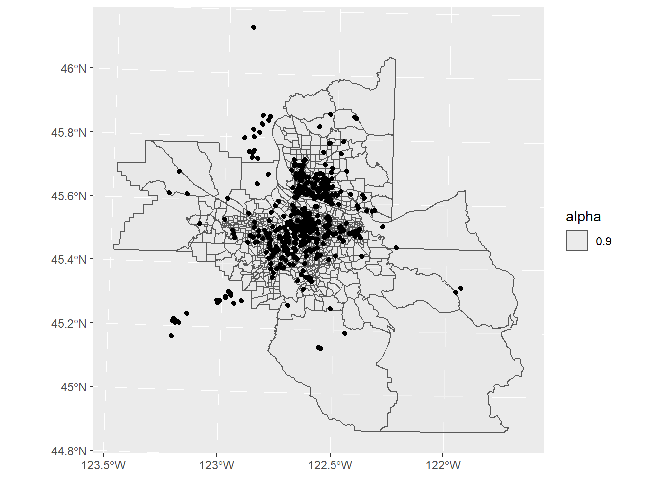
## # ... with 1 more variable: geometry <POINT [ft]>ggplot() +
geom_sf(data = taz_sf, aes(alpha=0.9)) +
geom_sf(data = portland94_sf)