10 Tidy Data
10.1 Readings
10.2 Tidy Data
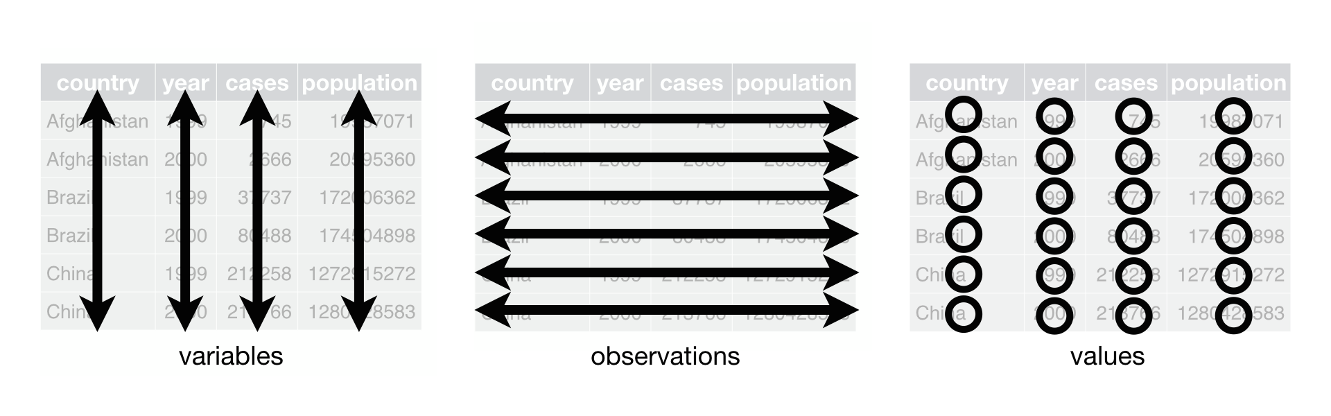
There are three interrelated rules which make a dataset tidy:
- Each variable must have its own column.
- Each observation must have its own row.
- Each value must have its own cell.
That interrelationship leads to an even simpler set of practical instructions:
- Put each dataset in a tibble.
- Put each variable in a column.
In this session, you will learn a consistent way to organise your data in R, an organisation called tidy data. Getting your data into this format requires some upfront work, but that work pays off in the long term. Once you have tidy data and the tidy tools provided by packages in the tidyverse, you will spend much less time munging data from one representation to another, allowing you to spend more time on the analytic questions at hand. This session will give you a practical introduction to tidy data and the accompanying tools in the tidyr package.
10.3 Lesson
table1 - table4 (loaded with the tidyverse package) below shows the same data organised in four different ways. Each dataset shows the same values of four variables country, year, population, and cases, but each dataset organises the values in a different way:
library(tidyverse)## Loading tidyverse: ggplot2
## Loading tidyverse: tibble
## Loading tidyverse: tidyr
## Loading tidyverse: readr
## Loading tidyverse: purrr
## Loading tidyverse: dplyr## Conflicts with tidy packages ----------------------------------------------## filter(): dplyr, stats
## lag(): dplyr, statstable1## # A tibble: 6 x 4
## country year cases population
## <chr> <int> <int> <int>
## 1 Afghanistan 1999 745 19987071
## 2 Afghanistan 2000 2666 20595360
## 3 Brazil 1999 37737 172006362
## 4 Brazil 2000 80488 174504898
## 5 China 1999 212258 1272915272
## 6 China 2000 213766 1280428583table2## # A tibble: 12 x 4
## country year type count
## <chr> <int> <chr> <int>
## 1 Afghanistan 1999 cases 745
## 2 Afghanistan 1999 population 19987071
## 3 Afghanistan 2000 cases 2666
## 4 Afghanistan 2000 population 20595360
## 5 Brazil 1999 cases 37737
## 6 Brazil 1999 population 172006362
## 7 Brazil 2000 cases 80488
## 8 Brazil 2000 population 174504898
## 9 China 1999 cases 212258
## 10 China 1999 population 1272915272
## 11 China 2000 cases 213766
## 12 China 2000 population 1280428583table3## # A tibble: 6 x 3
## country year rate
## * <chr> <int> <chr>
## 1 Afghanistan 1999 745/19987071
## 2 Afghanistan 2000 2666/20595360
## 3 Brazil 1999 37737/172006362
## 4 Brazil 2000 80488/174504898
## 5 China 1999 212258/1272915272
## 6 China 2000 213766/1280428583# Spread across two tibbles
table4a # cases## # A tibble: 3 x 3
## country `1999` `2000`
## * <chr> <int> <int>
## 1 Afghanistan 745 2666
## 2 Brazil 37737 80488
## 3 China 212258 213766table4b # population## # A tibble: 3 x 3
## country `1999` `2000`
## * <chr> <int> <int>
## 1 Afghanistan 19987071 20595360
## 2 Brazil 172006362 174504898
## 3 China 1272915272 1280428583These are all representations of the same underlying data, but they are not equally easy to use. One dataset, the tidy dataset, will be much easier to work with inside the tidyverse.
10.3.1 Spreading and gathering
The principles of tidy data seem so obvious that you might wonder if you’ll ever encounter a dataset that isn’t tidy. Unfortunately, however, most data that you will encounter will be untidy. There are two main reasons:
Most people aren’t familiar with the principles of tidy data, and it’s hard to derive them yourself unless you spend a lot of time working with data.
Data is often organised to facilitate some use other than analysis. For example, data is often organised to make entry as easy as possible.
This means for most real analyses, you’ll need to do some tidying. The first step is always to figure out what the variables and observations are. Sometimes this is easy; other times you’ll need to consult with the people who originally generated the data. The second step is to resolve one of two common problems:
One variable might be spread across multiple columns.
One observation might be scattered across multiple rows.
Typically a dataset will only suffer from one of these problems; it’ll only suffer from both if you’re really unlucky! To fix these problems, you’ll need the two most important functions in tidyr: gather() and spread().
10.3.1.1 Gathering
A common problem is a dataset where some of the column names are not names of variables, but values of a variable. Take table4a: the column names 1999 and 2000 represent values of the year variable, and each row represents two observations, not one.
table4a## # A tibble: 3 x 3
## country `1999` `2000`
## * <chr> <int> <int>
## 1 Afghanistan 745 2666
## 2 Brazil 37737 80488
## 3 China 212258 213766To tidy a dataset like this, we need to gather those columns into a new pair of variables. To describe that operation we need three parameters:
The set of columns that represent values, not variables. In this example, those are the columns
1999and2000.The name of the variable whose values form the column names. I call that the
key, and here it isyear.The name of the variable whose values are spread over the cells. I call that
value, and here it’s the number ofcases.
Together those parameters generate the call to gather():
table4a %>%
  gather(`1999`, `2000`, key = "year", value = "cases")
## # A tibble: 6 x 3
## country year cases
## <chr> <chr> <int>
## 1 Afghanistan 1999 745
## 2 Brazil 1999 37737
## 3 China 1999 212258
## 4 Afghanistan 2000 2666
## 5 Brazil 2000 80488
## 6 China 2000 213766The columns to gather are specified with dplyr::select() style notation. Here there are only two columns, so we list them individually. Note that “1999” and “2000” are non-syntactic names so we have to surround them in backticks. To refresh your memory of the other ways to select columns, see select.
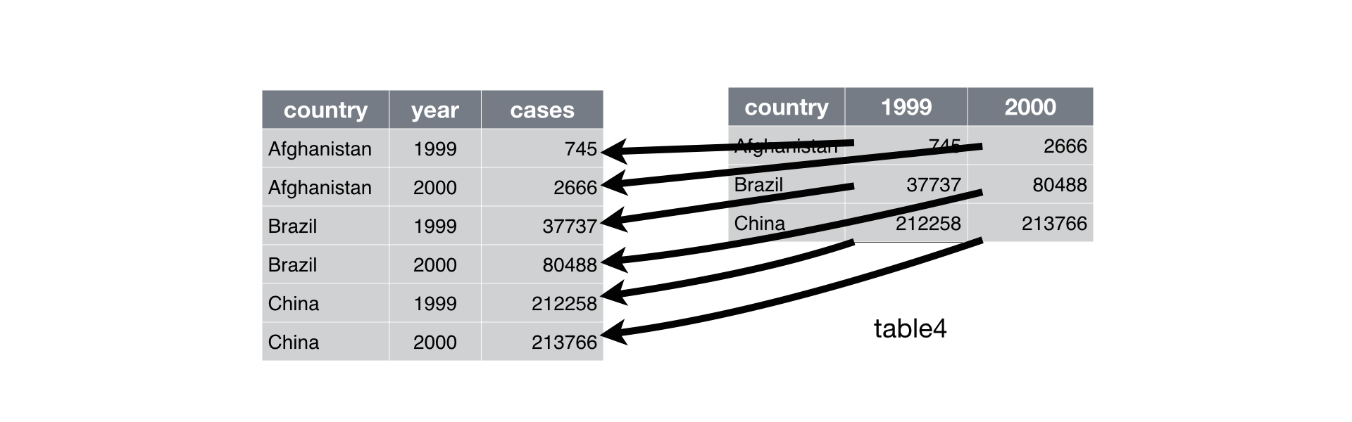
Figure 10.1: Gathering table4 into a tidy form.
In the final result, the gathered columns are dropped, and we get new key and value columns. Otherwise, the relationships between the original variables are preserved. Visually, this is shown in Figure 10.1. We can use gather() to tidy table4b in a similar fashion. The only difference is the variable stored in the cell values:
table4b %>%
  gather(`1999`, `2000`, key = "year", value = "population")
## # A tibble: 6 x 3
## country year population
## <chr> <chr> <int>
## 1 Afghanistan 1999 19987071
## 2 Brazil 1999 172006362
## 3 China 1999 1272915272
## 4 Afghanistan 2000 20595360
## 5 Brazil 2000 174504898
## 6 China 2000 1280428583To combine the tidied versions of table4a and table4b into a single tibble, we need to use dplyr::left_join(), which you’ll learn about in [relational data].
tidy4a <- table4a %>%
  gather(`1999`, `2000`, key = "year", value = "cases")
tidy4b <- table4b %>%
  gather(`1999`, `2000`, key = "year", value = "population")
left_join(tidy4a, tidy4b)
## Joining, by = c("country", "year")## # A tibble: 6 x 4
## country year cases population
## <chr> <chr> <int> <int>
## 1 Afghanistan 1999 745 19987071
## 2 Brazil 1999 37737 172006362
## 3 China 1999 212258 1272915272
## 4 Afghanistan 2000 2666 20595360
## 5 Brazil 2000 80488 174504898
## 6 China 2000 213766 128042858310.3.1.2 Spreading
Spreading is the opposite of gathering. You use it when an observation is scattered across multiple rows. For example, take table2: an observation is a country in a year, but each observation is spread across two rows.
table2## # A tibble: 12 x 4
## country year type count
## <chr> <int> <chr> <int>
## 1 Afghanistan 1999 cases 745
## 2 Afghanistan 1999 population 19987071
## 3 Afghanistan 2000 cases 2666
## 4 Afghanistan 2000 population 20595360
## 5 Brazil 1999 cases 37737
## 6 Brazil 1999 population 172006362
## 7 Brazil 2000 cases 80488
## 8 Brazil 2000 population 174504898
## 9 China 1999 cases 212258
## 10 China 1999 population 1272915272
## 11 China 2000 cases 213766
## 12 China 2000 population 1280428583To tidy this up, we first analyse the representation in similar way to gather(). This time, however, we only need two parameters:
The column that contains variable names, the
keycolumn. Here, it’stype.The column that contains values forms multiple variables, the
valuecolumn. Here it’scount.
Once we’ve figured that out, we can use spread(), as shown programmatically below, and visually in Figure 10.2.
spread(table2, key = type, value = count)## # A tibble: 6 x 4
## country year cases population
## * <chr> <int> <int> <int>
## 1 Afghanistan 1999 745 19987071
## 2 Afghanistan 2000 2666 20595360
## 3 Brazil 1999 37737 172006362
## 4 Brazil 2000 80488 174504898
## 5 China 1999 212258 1272915272
## 6 China 2000 213766 1280428583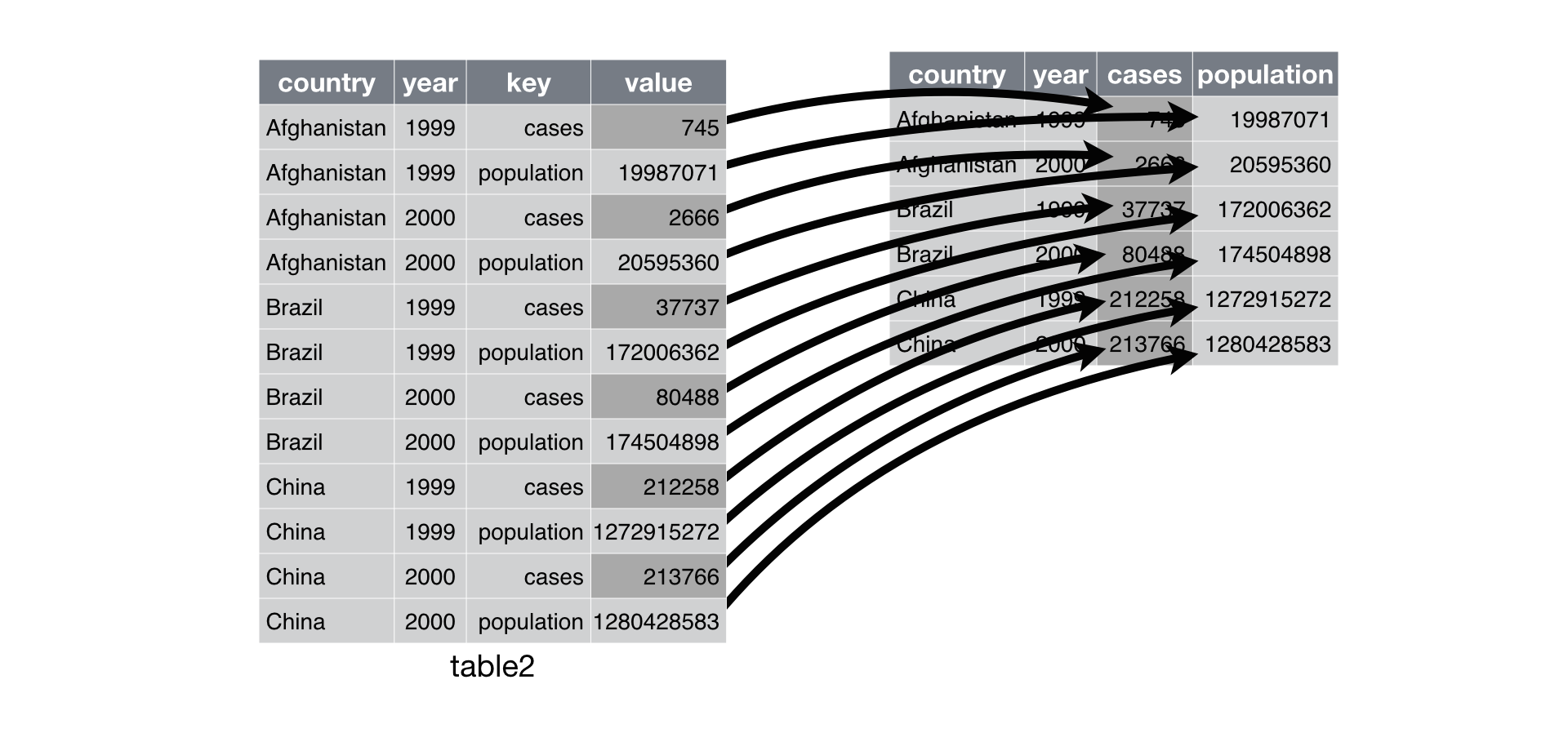
Figure 10.2: Spreading table2 makes it tidy
As you might have guessed from the common key and value arguments, spread() and gather() are complements. gather() makes wide tables narrower and longer; spread() makes long tables shorter and wider.
10.3.2 Separating and uniting
So far you’ve learned how to tidy table2 and table4, but not table3. table3 has a different problem: we have one column (rate) that contains two variables (cases and population). To fix this problem, we’ll need the separate() function. You’ll also learn about the complement of separate(): unite(), which you use if a single variable is spread across multiple columns.
10.3.2.1 Separate
separate() pulls apart one column into multiple columns, by splitting wherever a separator character appears. Take table3:
table3## # A tibble: 6 x 3
## country year rate
## * <chr> <int> <chr>
## 1 Afghanistan 1999 745/19987071
## 2 Afghanistan 2000 2666/20595360
## 3 Brazil 1999 37737/172006362
## 4 Brazil 2000 80488/174504898
## 5 China 1999 212258/1272915272
## 6 China 2000 213766/1280428583The rate column contains both cases and population variables, and we need to split it into two variables. separate() takes the name of the column to separate, and the names of the columns to separate into, as shown in Figure 10.3 and the code below.
table3 %>%
  separate(rate, into = c("cases", "population"))
## # A tibble: 6 x 4
## country year cases population
## * <chr> <int> <chr> <chr>
## 1 Afghanistan 1999 745 19987071
## 2 Afghanistan 2000 2666 20595360
## 3 Brazil 1999 37737 172006362
## 4 Brazil 2000 80488 174504898
## 5 China 1999 212258 1272915272
## 6 China 2000 213766 1280428583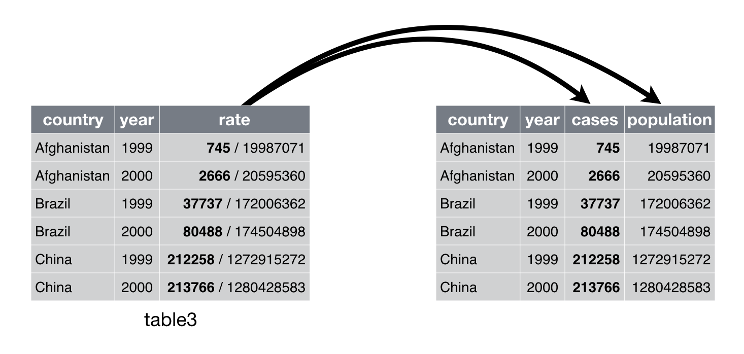
Figure 10.3: Separating table3 makes it tidy
By default, separate() will split values wherever it sees a non-alphanumeric character (i.e. a character that isn’t a number or letter). For example, in the code above, separate() split the values of rate at the forward slash characters. If you wish to use a specific character to separate a column, you can pass the character to the sep argument of separate(). For example, we could rewrite the code above as:
table3 %>%
  separate(rate, into = c("cases", "population"), sep = "/")
(Formally, sep is a regular expression, which you’ll learn more about in [strings].)
Look carefully at the column types: you’ll notice that case and population are character columns. This is the default behaviour in separate(): it leaves the type of the column as is. Here, however, it’s not very useful as those really are numbers. We can ask separate() to try and convert to better types using convert = TRUE:
table3 %>%
  separate(rate, into = c("cases", "population"), convert = TRUE)
## # A tibble: 6 x 4
## country year cases population
## * <chr> <int> <int> <int>
## 1 Afghanistan 1999 745 19987071
## 2 Afghanistan 2000 2666 20595360
## 3 Brazil 1999 37737 172006362
## 4 Brazil 2000 80488 174504898
## 5 China 1999 212258 1272915272
## 6 China 2000 213766 1280428583You can also pass a vector of integers to sep. separate() will interpret the integers as positions to split at. Positive values start at 1 on the far-left of the strings; negative value start at -1 on the far-right of the strings. When using integers to separate strings, the length of sep should be one less than the number of names in into.
You can use this arrangement to separate the last two digits of each year. This make this data less tidy, but is useful in other cases, as you’ll see in a little bit.
table3 %>%
  separate(year, into = c("century", "year"), sep = 2)
## # A tibble: 6 x 4
## country century year rate
## * <chr> <chr> <chr> <chr>
## 1 Afghanistan 19 99 745/19987071
## 2 Afghanistan 20 00 2666/20595360
## 3 Brazil 19 99 37737/172006362
## 4 Brazil 20 00 80488/174504898
## 5 China 19 99 212258/1272915272
## 6 China 20 00 213766/128042858310.3.2.2 Unite
unite() is the inverse of separate(): it combines multiple columns into a single column. You’ll need it much less frequently than separate(), but it’s still a useful tool to have in your back pocket.
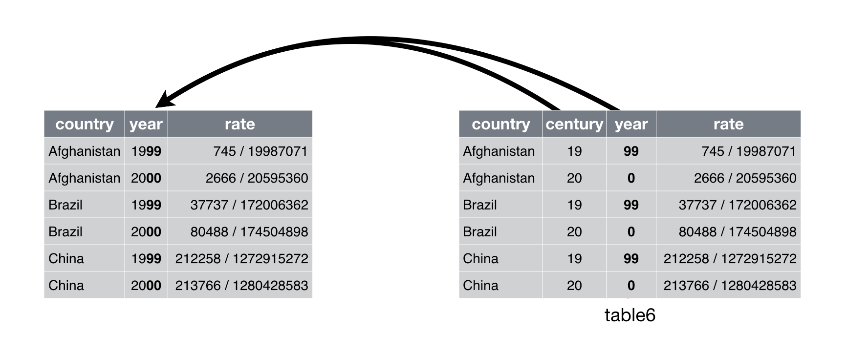
Figure 10.4: Uniting table5 makes it tidy
We can use unite() to rejoin the century and year columns that we created in the last example. That data is saved as tidyr::table5. unite() takes a data frame, the name of the new variable to create, and a set of columns to combine, again specified in dplyr::select() style:
table5 %>%
  unite(new, century, year)
## # A tibble: 6 x 3
## country new rate
## * <chr> <chr> <chr>
## 1 Afghanistan 19_99 745/19987071
## 2 Afghanistan 20_00 2666/20595360
## 3 Brazil 19_99 37737/172006362
## 4 Brazil 20_00 80488/174504898
## 5 China 19_99 212258/1272915272
## 6 China 20_00 213766/1280428583In this case we also need to use the sep argument. The default will place an underscore (_) between the values from different columns. Here we don’t want any separator so we use "":
table5 %>%
  unite(new, century, year, sep = "")
## # A tibble: 6 x 3
## country new rate
## * <chr> <chr> <chr>
## 1 Afghanistan 1999 745/19987071
## 2 Afghanistan 2000 2666/20595360
## 3 Brazil 1999 37737/172006362
## 4 Brazil 2000 80488/174504898
## 5 China 1999 212258/1272915272
## 6 China 2000 213766/128042858310.4 Exercise
- Are the bike counts data for the two bridges tidy data?
- If not, why not? And how can we tidy it?
- After tidying the bike counts, using functions in the
tidyrpackage, create tables summarizing the average bike counts by bridge and day of week in two different formats:
| Bridge | Sun | Mon | Tue | Wed | Thur | Fri | Sat |
|---|---|---|---|---|---|---|---|
| Hawthorne | |||||||
| Tilikum |
| Day of Week | Hawthorne | Tilikum |
|---|---|---|
| Fri | ||
| Mon | ||
| Sat | ||
| Sun | ||
| Thur | ||
| Tue | ||
| Wed |