8 Part II: Overview and Introduction

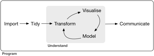
Data Science is a discipline that combines computing with statistics. A data analysis problem is solved in a series of data-centric steps: data acquisition and representation (Import), data cleaning (Tidy), and an iterative sequence of data transformation (Transform), data modelling (Model) and data visualization (Visualize). The end result of the process is to communicate insights obtained from the data (Communicate). Part II of this class will take you through all the steps in the process and will teach you how to approach such problems in a systematic manner. You will learn how to design data analysis pipelines as well as how to implement data analysis pipelines in R. The class will also emphasize how elegant code leads to reproducible science.

8.1 Part II: tidyverse work flow

8.2 Readings

R4DS Chapter 1

8.3 The tidyverse workflow

First you must import your data into R. This typically means that you take data stored in a file, database, or web API, and load it into a data frame in R. If you can’t get your data into R, you can’t do data science on it!

Once you’ve imported your data, it is a good idea to tidy it. Tidying your data means storing it in a consistent form that matches the semantics of the dataset with the way it is stored. In brief, when your data is tidy, each column is a variable, and each row is an observation. Tidy data is important because the consistent structure lets you focus your struggle on questions about the data, not fighting to get the data into the right form for different functions.

Once you have tidy data, a common first step is to transform it. Transformation includes narrowing in on observations of interest (like all people in one city, or all data from the last year), creating new variables that are functions of existing variables (like computing velocity from speed and time), and calculating a set of summary statistics (like counts or means). Together, tidying and transforming are called wrangling, because getting your data in a form that’s natural to work with often feels like a fight!

Once you have tidy data with the variables you need, there are two main engines of knowledge generation: visualisation and modelling. These have complementary strengths and weaknesses so any real analysis will iterate between them many times.

Visualisation is a fundamentally human activity. A good visualisation will show you things that you did not expect, or raise new questions about the data. A good visualisation might also hint that you’re asking the wrong question, or you need to collect different data. Visualisations can surprise you, but don’t scale particularly well because they require a human to interpret them.

Models are complementary tools to visualisation. Once you have made your questions sufficiently precise, you can use a model to answer them. Models are a fundamentally mathematical or computational tool, so they generally scale well. Even when they don’t, it’s usually cheaper to buy more computers than it is to buy more brains! But every model makes assumptions, and by its very nature a model cannot question its own assumptions. That means a model cannot fundamentally surprise you.

The last step of data science is communication, an absolutely critical part of any data analysis project. It doesn’t matter how well your models and visualisation have led you to understand the data unless you can also communicate your results to others.

Surrounding all these tools is programming. Programming is a cross-cutting tool that you use in every part of the project. You don’t need to be an expert programmer to be a data scientist, but learning more about programming pays off because becoming a better programmer allows you to automate common tasks, and solve new problems with greater ease.

You’ll use these tools in every data science project, but for most projects they’re not enough. There’s a rough 80-20 rule at play; you can tackle about 80% of every project using the tools that you’ll learn in this book, but you’ll need other tools to tackle the remaining 20%. Throughout this book we’ll point you to resources where you can learn more.

8.4 The tidyverse packages

Website: http://www.tidyverse.org/packages/
Install with install.packages("tidyverse")

8.5 Pipe operator

%>% pipes an object forward into a function or call expression

Basic piping
- x %>% f is equivalent to f(x)
- x %>% f(y) is equivalent to f(x, y)
- x %>% f %>% g %>% h is equivalent to h(g(f(x)))
Using %>% with unary function calls

require(tidyverse)

## Loading required package: tidyverse

## Loading tidyverse: ggplot2
## Loading tidyverse: tibble
## Loading tidyverse: tidyr
## Loading tidyverse: readr
## Loading tidyverse: purrr
## Loading tidyverse: dplyr

## Conflicts with tidy packages ----------------------------------------------

## filter(): dplyr, stats
## lag():    dplyr, stats

iris %>% head

##   Sepal.Length Sepal.Width Petal.Length Petal.Width Species
## 1          5.1         3.5          1.4         0.2  setosa
## 2          4.9         3.0          1.4         0.2  setosa
## 3          4.7         3.2          1.3         0.2  setosa
## 4          4.6         3.1          1.5         0.2  setosa
## 5          5.0         3.6          1.4         0.2  setosa
## 6          5.4         3.9          1.7         0.4  setosa

iris %>% tail

##     Sepal.Length Sepal.Width Petal.Length Petal.Width   Species
## 145          6.7         3.3          5.7         2.5 virginica
## 146          6.7         3.0          5.2         2.3 virginica
## 147          6.3         2.5          5.0         1.9 virginica
## 148          6.5         3.0          5.2         2.0 virginica
## 149          6.2         3.4          5.4         2.3 virginica
## 150          5.9         3.0          5.1         1.8 virginica

Placing lhs as the first argument in rhs call

## What are the outputs for these two lines?
3 %>% `-`(4)
iris %>% head(5)
iris %>% tail(5)

Placing lhs elsewhere in rhs call

## What are the outputs for these
3 %>% `-`(4, .)
4 %>% c("A", "B", "C", "D", "E")[.]

More information available at: http://magrittr.tidyverse.org/

8.5.1 RStudio keyboard shortcut for `%>%`

ctrl-Shift-M (Windows)
Command-Shift-M (Mac)

8.6 Class project

For the class project for Part II, you are expected to follow the tidyverse work flow and use the tidyverse suite of packages to conduct an analytic project using data of your choice. Your project should involve these steps:

Data importing and tidying;
Data transformation;
Data Visualization;
[Optional] Data modeling;
[Optional] Reproducible reporting.

You can use data from your current work or continue a project you have been working on. Take the feasibility of completing in a week into consideration when selecting project ideas.

If you don’t have a feasible project idea at the moment, consider continuing to analyze the bike counts data on Hawthorne Bridge and Tilikum Crossing from Part I. Daily traffic counts data for these two bridges can be found here.

Sample analytic questions are:

After accounting for seasonal variation, is there a trend in bike traffic across these two bridges?
How was the bike traffic affected by weather (temperature, precipitation, etc)?
Was the bike traffic on the Hawthorne Bridge affected by the opening of Tilikum Crossing?

You can work on any one or all of these questions with visualization and/or modeling after you import, tidy and transform the data when necessary.